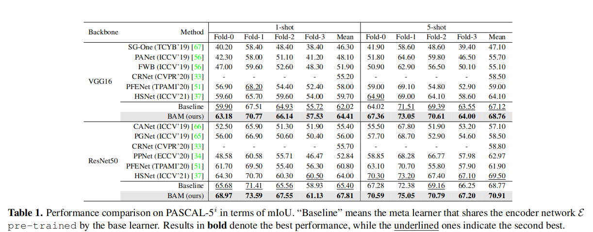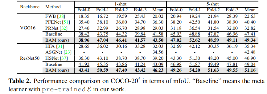
Learning What Not to Segment A New Perspective on Few-Shot Segmentation

I read the paper in the first month when I came in MiLab. However, at that time I could not recognize the quality of this method (I usually don’t read the experiment carefully). It appeared when I was reading another paper called “Holistic Prototype Activation for Few-Shot Segmentation”. The HPA performs well but can not beat BAM (although HPA has less parameter to train, obviously). So I decided to read this paper again.

ABSTRACT & INTRODUCTION

Previous problem:

the trained models are biased towards the seen classes instead of being ideally class-agnostic

Contribution

BAM, i.e., base and the meta has two branches, allowing model to learn what not to segment and what to segmentation, respectively.
Design a special loss in order to train two branches suitably.
Extend the proposed approach to a more challenging setting, which simultaneously identifies the targets of base and novel classes.

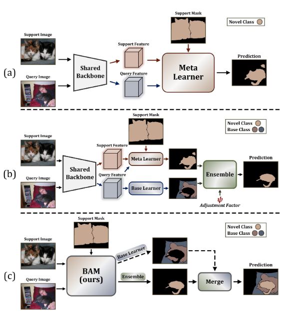
In the following image, (a) is a classical method to address FSS task; (b) is BAM approach; (c) is the extension of BAM

METHOD

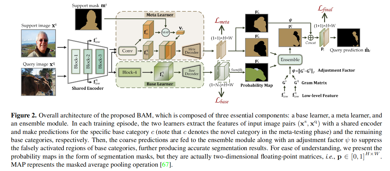
They adopt two stage training method, which means they train base learner and meta learner separately.

BASE LEARNER

Query image goes through four ResNet blocks and becomes intermediate feature maps $f_b^q$. Then the decoder network $D_b$ yields the prediction result. $N_b$ represents the number of base categories. $$ P_b = softmax(D_b(f_b^q)) \in R^{(1+N_b)\times H\times W} $$ Loss can be defined as $$ L_{base} = \frac{1}{n_{bs}}\sum_{i=1}^{n_{bs}}CE(P_{b;i},m^q_{b;i}) $$ It is worth noting that they do not employ the general FSS learning paradigm (update the parameter in each episode). And they train the base learner independently. They explain as follow:

It is unrealistic to additionally build such a large network on the basis of the original few-shot model, which will introduce too many parameters and slow down the inference speed.
It is unknown whether the base learner can be trained well with the episodic learning paradigm, so a two stage training strategy is eventually adopted.

In the ablation study, it shows that with two stage train, the model can perform better.

META LEARNER

This part is highly resemble similar to CANet, employing “expand & concatenate” operations. The loss can be described as $$ L_{meta} = \frac{1}{n_e}\sum_{i=1}^{n_e}BCE(p_{m;i},m_i^q) $$ , when $n_e$ denotes the number of training episodes in each batch

Ensemble

This part is designed to leverage the low-level feature to adjust the coarse predictions which is derived from meta learner.

Firstly, we calculate the overall indicator $\psi$ for guiding the adjustment process: $$ A_s = F_{reshape}(f_{low}^s) \in R^{C_1\times N},\ G^s = A_sA^T \in R^{C_1\times C_1} $$ $G^s$ should be denoted as Gram matrix, BTW.

Gram matrix can be regarded as eccentric covariance matrix between features. Every number in gram matrix describe the relation between every two feature, about which two features appear simultaneously, which two features just offset from each other, etc.

$$ \psi =||G^s - G^q||_F $$

$||\ ||_F$ denotes the Frobenius norm of the input metirx.

After that, the final segmentation pridections $P_f$ can be described as follow: $$ p_f^0 = F_{ensemble}(F_\psi(p_m^0),p_b^f), \ p_f=p_f^0(+)F_\psi(p_m^1) $$ where $p_m$,$p_b$ denote the predictions of the meta learner and base learner respectively. The superscript “0” and “1” represent the background and foreground respectively. Both $F_ψ$ and $F_{ensemble}$ are 1×1 convolution operations with specific initial parameters.

LOSS

$$ L=L_{final} + \lambda L_{meta} \ L_{final} = \frac{1}{n_e}\sum_{i=1}^{n_e}BCE(p_i^q,m_i^q) $$

where $L_{meta}$ is the loss function of the meta learner defined in the meta learner stage.